The Shooting Method
by R. Grothmann
We show how to solve a boundary value problem with the shooting method.
To get an example with a known solution, we solve
![]()
using Maxima.
>&ode2('diff(y,x,2)=y+'diff(y,x)*x,y,x); sol &= rhs(%)
                              2
                             x
                             --                      2
                             2         x            x
               sqrt(pi) %k1 E   erf(-------)        --
                                    sqrt(2)         2
               ----------------------------- + %k2 E
                          sqrt(2)
Now we solve the boundary value problem y(0)=y(1)=1.
>&solve([at(sol,x=0)=1,at(sol,x=1)=1],[%k1,%k2]);  ...
   function y(x) &= sol with %[1]
                                     2
                                    x
                                    -- - 1/2                  2
                                    2               x        x
       (sqrt(2) - sqrt(2) sqrt(E)) E         erf(-------)    --
                                                 sqrt(2)     2
       -------------------------------------------------- + E
                                     1
                      sqrt(2) erf(-------)
                                  sqrt(2)
Indeed, this is the solution.
>&float(y(0)), &float(y(1)),
                                 1.0


                                 1.0
The derivative at 0.
>&float(diffat(y(x),x=0))
- 0.45986222928643
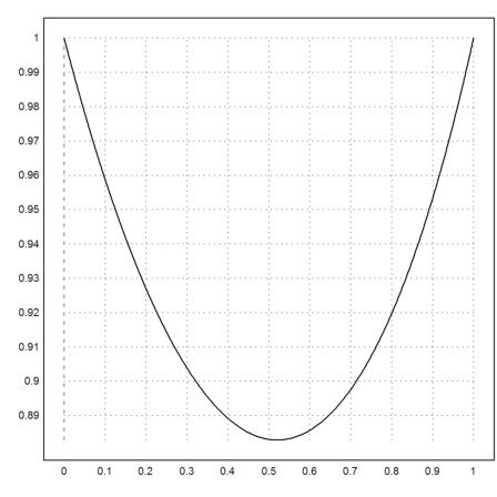
Plot the solution in Euler.
>plot2d(&y(x),0,1):
Now we want to solve the differential equation in Euler.
First we rewrite the equation as a system of two differential equations of order 1. So we set u[1]=y, u[2]=y'.
>function f(x,u) := [u[2],u[1]+x*u[2]]
For a try, we start with the correct solution u(0)=1, u(1)=y'(0).
>u0=[1,mxmeval("diffat(y(x),x=0)")];
We get the correct value for y(1)=u_1(1).
>x=0:0.01:1; u=adaptiverunge("f",x,u0); u[1,-1]
1
To solve the boundary value problem from sratch, we define a function shoot, which maps y'(0) to y(1).
>function map shoot (dy0) := adaptiverunge("f",[0,1],[1,dy0])[1,2]
For the correct y'(0), the solution for y(1) is obtained.
>shoot(mxmeval("diffat(y(x),x=0)"))
1
>plot2d("shoot",-2,2):
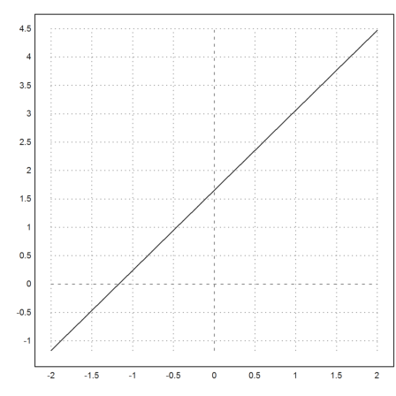
To find the correct value for y'(0), we can use the bisection method.
>bisect("shoot",-2,2,y=1)
-0.459862229286
Or the secant method.
>solve("shoot",0,y=1)
-0.459862229287